Graph
- Graphs are collections of vertices and edges.
class Vertex:
 def __init__(self, key):
  self.id = key
  self.connected_to = {}

 def add_neighbor(self, n, w):
  self.connected_to[n] = w

 def get_connections(self):
  return self.connected_to.keys()

 def get_id(self):
  return self.id

 def get_weight(self, n):
  return self.connected_to[n]

 def __str__(self):
  return str(self.id)

class Graph:
 def __init__(self):
  self.size = 0
  self.master_list = {}

 def add_vertex(self, key):
  self.size += 1
  vertex = Vertex(key)
  self.master_list[key] = vertex
  return vertex

 def get_vertex(self, n):
  if n in self.master_list:
   return self.master_list[n]
  return None

 def add_edge(self, u, v, weight=0):
  if u not in self.master_list:
   self.add_vertex(u)
  if v not in self.master_list:
   self.add_vertex(v)
  self.master_list[u].add_neighbor(self.add_vertex(v), weight)

 def get_vertices(self):
  return self.master_list.keys()

 def __iter__(self):
  return iter(self.master_list.values())

 def __contains__(self, n):
  if n in self.master_list:
   return True
  return False

if __name__ == "__main__":
 graph = Graph()
 for value in range(6):
  graph.add_vertex(value)

 graph.add_edge(0, 1, 5)

 for vertex in graph:
  print(vertex)
The categories of graph problems
- Existence: Problems that attempt to determine if a path, a vertex, or a set exists, particularly if there is a constraint.
- Construction: Given a set of paths and vertices with a constraint, how to construct a graph.
- Enumeration: Problems that attempt to determine how many vertices and edges exist, given a set of constraints.
- Optimization: Problems that attempt to find the shortest path between two nodes.
Articulation points
- An articulation point/cut vertex is any node in a graph whose removal increases the number of connected components.
- It often hints at the weak points, bottlenecks, and vulnerabilities.
Breadth-First Search
- Data structure: Queue
- Aim: Graph traversal
- Runtime: $O(V+E)$
Algorithm:
- Start from a node.
- Visit all its children.
- Move on to the grandchildren and continue this process until there is no unvisited vertex.
graph = {
    'A' : ['B', 'C'],
    'B' : ['D', 'E'],
    'C' : ['F'],
    'D' : [],
    'E' : ['F'],
    'F' : []
}

def bfs(graph, node):
    queue = [node]
    visited = [node]
    while queue:
        popped_node = queue.pop(0)
        for neighbour in graph[popped_node]:
            if neighbour not in visited:
                queue.append(neighbour)
                visited.append(neighbour)
    return visited

visited = bfs(graph, 'A')
print(visited)
Applications
Connected components
- In connected graphs, there is a path between any two vertices.
- A connected component of an undirected graph is a maximal set of vertices such that there is a path between every pair of vertices.
Two-coloring graphs
- The vertex colouring problem seeks to assign a label to each vertex of a graph such that no edge links any two vertices of the same colour.
- The goal is to use as few colours as possible.
- Scheduling applications
- Register allocation in compilers
Bipartite matching
-
A matching in a graph $G = (V,E)$ is a subset of edges $E’ \subset E$ such that no two edges of $E’$ share a vertex.
-
To solve bipartite matching, we constructed a special network flow graph such that the maximum flow corresponds to a matching having the largest number of edges.
Connected Components
- We can use DFS to identify the connected components.
- Assign an integer value to each group to be able to tell them apart.
Algorithm:
- Label each node using a number within the range [0,n), where n is the number of nodes.
- Start DFS at each visited node and mark all reachable nodes as being part of the same component.
class Graph:
  def __init__(self, num_vertex: int):
    self.num_vertex = num_vertex
    self.adj_list = [[] for _ in range(num_vertex)]

  def add_edge(self, from_node: int, to_node: int) -> None:
    self.adj_list[from_node].append(to_node)
    self.adj_list[to_node].append(from_node)

  def dfs(self, node, component, visited):
    visited[node] = True
    component.append(node)
    for neighbour in self.adj_list[node]:
      if visited[neighbour] == False:
        self.dfs(neighbour, component, visited)

  def connected_components(self):
    all_components = []
    visited = [ False for _ in range(self.num_vertex) ]
    for i in range(self.num_vertex):
      if visited[i] == False:
        component = []
        self.dfs(i, component, visited)
        all_components.append(component)
    return all_components

if __name__ == "__main__":
  graph = Graph(5)

  graph.add_edge(1,0)
  graph.add_edge(2,3)
  graph.add_edge(3,0)

  print(graph.connected_components())
Connectivity
- The smallest number of vertices whose deletion will disconnect the graph.
Solution
- Union find data structure
- Any search algorithm (DFS), etc.
Cycle detection
Cycle detection in a directed graph
from collections import defaultdict

class Graph():
    def __init__(self, order):
        self.graph = defaultdict(list)
        self.order = order

    def addEdge(self, u, v):
        self.graph[u].append(v)

    def is_cyclic_helper(self, node, visited, stack):
        visited[node] = True
        stack[node] = True
        for neighbour in self.graph[node]:
            if visited[neighbour] == False:
                if self.is_cyclic_helper(neighbour, visited, stack):
                    return True
            elif stack[neighbour] == True:
                return True
        stack[node] = False
        return False

    def is_cyclic(self):
        visited = [ False for _ in range(self.order) ]
        stack = [ False for _ in range(self.order) ] # may be needed for subgraphs
        for node in range(self.order): # helpful for disconnected graphs
            if visited[node] == False:
                if self.is_cyclic_helper(node, visited, stack):
                    return True
        return False

if __name__ == "__main__":
    graph = Graph(4)

    graph.addEdge(0, 1)
    graph.addEdge(0, 2)
    graph.addEdge(1, 2)
    graph.addEdge(2, 0)
    graph.addEdge(2, 3)
    graph.addEdge(3, 3)
    print(graph.is_cyclic())

    # graph.addEdge(0, 1)
    # graph.addEdge(0, 2)
    # print(graph.is_cyclic())
Cycle detection in an undirected graph
from collections import defaultdict

class Graph():
    def __init__(self, order):
        self.graph = defaultdict(list)
        self.order = order

    def addEdge(self, u, v):
        self.graph[u].append(v)
        self.graph[v].append(u)

    def is_cyclic_helper(self, node, visited, parent):
        visited[node] = True
        for neighbour in self.graph[node]:
            if visited[neighbour] == False:
                if self.is_cyclic_helper(neighbour, visited, node):
                    return True
            elif parent != neighbour:
                return True
        return False

    def is_cyclic(self):
        visited = [ False for _ in range(self.order) ]
        for node in range(self.order): # helpful for disconnected graphs
            if visited[node] == False:
                if self.is_cyclic_helper(node, visited, -1):
                    return True
        return False


if __name__ == "__main__":
    graph = Graph(4)

    graph.addEdge(0, 1)
    graph.addEdge(0, 2)
    graph.addEdge(1, 2)
    print(graph.is_cyclic())

    # graph.addEdge(0, 1)
    # graph.addEdge(0, 2)
    # print(graph.is_cyclic())
Depth First Search (DFS)
- Data structure: Stack_
- Aim: Graph traversal
- Runtime: $O(V+E)$
graph = {
    'A' : ['B','C'],
    'B' : ['D', 'E'],
    'C' : ['F'],
    'D' : [],
    'E' : ['F'],
    'F' : []
}

# preorder
# def dfs_iterative(graph, node, visited):
#     stack = [node]
#     while stack:
#         popped_item = stack.pop()
#         if popped_item not in visited:
#             visited.append(popped_item) # pre
#             for neighbour in graph[popped_item]:
#                 if neighbour not in visited:
#                     stack.append(neighbour)
#     return visited

# post-order
def dfs_iterative(graph: Dict[int, int], start_node: int) -> List[int]:
    stack = [start_node]
    visited = []
    while stack:
        popped_node = stack.pop()
        if popped_node not in visited:
            for neighbour in graph[popped_node]:
                if neighbour not in visited:
                    stack.append(neighbour)
            visited.append(popped_node)
    return visited

visited = dfs_iterative(graph, 'A')
print(visited)

# inorder bst traversal iterative
# class Node:
#     def __init__(self, val):
#         self.val = val
#         self.left = None
#         self.right = None

#     def inorder_iterative_dfs(root):
#         if not root:
#             return

#         stack = []
#         while True:
#             if root:
#                 stack.append(root)
#                 root = root.left
#             else:
#                 if not stack:
#                     break
#                 root = stack.pop()
#                 print(root.val)
#                 root = root.right


# root = Node(10)
# root.left = Node(0)
# root.left.left = Node(5)
# root.left.right = Node(6)
# root.right = Node(-10)
# root.right.right = Node(11)

# Node.inorder_iterative_dfs(root)
DFS algorithm
- Dig deep down into paths branching off of the starting point until it reaches a point where either there is no more edge forward or meets a previously visited vertex. We don’t want to revisit it.
DFS recursive
graph = {
    'A' : ['B','C'],
    'B' : ['D', 'E'],
    'C' : ['F'],
    'D' : [],
    'E' : ['F'],
    'F' : [],
    'G' : ['H'],
    'H' : [],
}

def dfs(graph, node, visited):
    if node not in visited:
        visited.append(node)
        for neighbour in graph[node]:
            dfs(graph, neighbour, visited)

# to traverse whole graph
visited = []
for node in graph:
    if node not in visited:
        dfs(graph, node, visited)

print(visited)
Applications of arrival and departure time of vertices
- Topological sorting
- Finding 2/3–(edge or vertex)–connected components
- Finding bridges in graphs
- Finding biconnectivity in graphs
- Detecting cycle in directed graphs
- Tarjan’s algorithm to find strongly connected components, etc.
from collections import defaultdict
from typing import List, Tuple

class Graph:
 def __init__(self, order: int, edges: List[Tuple[int, int]]):
  self.order = order
  self.adj_list = {}

  for (src, dest) in edges:
   if src not in self.adj_list:
    self.adj_list[src] = []
   if dest not in self.adj_list:
    self.adj_list[dest] = []

   self.adj_list[src].append(dest)

 def __repr__(self):
  out = []
  for s_node in self.adj_list:
   out.append(f"{s_node} -> ")
   for d_node in self.adj_list[s_node]:
    out.append(f"{d_node}, ")
   out.append('\n')
  return ''.join(out)

def dfs(graph: Graph, start_node: int, visited: List[int], arrival: List[int], departure: List[int], time: int) -> int:
 if start_node not in visited:
  time += 1
  arrival[start_node] = time
  visited.append(start_node)
  for neighbour in graph.adj_list[start_node]:
   time = dfs(graph, neighbour, visited, arrival, departure, time)
  time += 1
  departure[start_node] = time
 return time

if __name__ == "__main__":
 edges = [ (0, 1), (0, 2), (2, 3), (2, 4), (3, 1), (3, 5), (4, 5), (6, 7) ]
 graph = Graph(8, edges)
 visited, arrival, departure = [], {}, {}
 time = -1
 for node in graph.adj_list:
  if node not in visited:
   time = dfs(graph, node, visited, arrival, departure, time)

 for i in range(len(visited)):
  print(f"{visited[i]} - {arrival[i]} - {departure[i]}")
Directed Acycling Graph (DAG)
- DAG is a graph with directed edges and no cycle.
- A graph with a cycle cannot have a valid ordering.
- All rooted trees have topological ordering since they do not contain any cycles.
Directed graph
from typing import List, Tuple

class Graph:
    def __init__(self, edge_list: List[Tuple[int, int]], order: int):
        self.adj_list = {}
        for (src, dest) in edge_list:
            if src not in self.adj_list:
                self.adj_list[src] = []
            if dest not in self.adj_list:
                self.adj_list[dest] = []
            self.adj_list[src].append(dest)

    def __repr__(self):
        out = []
        for s_node in self.adj_list:
            out.append(f"{s_node} -> ")
            for d_node in self.adj_list[s_node]:
                out.append(f"{d_node}, ")
            out.append('\n')
        return ''.join(out)


if __name__ == '__main__':
    edge_list = [ (0,1), (1,2), (2,3), (0,2), (3,2), (4,5), (5,4) ]
    order = 6

    graph = Graph(edge_list, order)
    print(graph)
Disjoint set
class DisjointSet:

 def __init__(self, size):
  self.root = [ i for i in range(size) ]

 def find(self, x):

  if self.root[x] == x:
   return x

  self.root[x] = self.find(self.root[x])

  return self.root[x]

 def union(self, x, y):

  rootX = self.find(x)
  rootY = self.find(y)

  if rootX != rootY:
   self.root[rootY] = rootX

 def connected(self, x, y):
  return self.find(x) == self.find(y)

 def __str__(self):
  return str(self.root)

disjoint_set = DisjointSet(10)

disjoint_set.union(1, 2)
disjoint_set.union(1, 2)
disjoint_set.union(2, 5)
disjoint_set.union(5, 6)
disjoint_set.union(6, 7)
disjoint_set.union(3, 8)
disjoint_set.union(8, 9)
disjoint_set.union(9, 4)

print(disjoint_set)

print(disjoint_set.connected(1, 5))
Eulerian path
Eulerian Graph
-
A graph is considered Eulerian if you can start at a vertex, traverse through every edge only once, and return to the same vertex you started at.
-
A graph is Eulerian if and only if each vertex has an even degree.
Finding Bridges
- A bridge/cut edge is any edge in a graph whose removal increases the number of connected components.
- It often hints at the weak points, bottlenecks, and vulnerabilities.
Graph colouring
- Coloring nodes means assigning the same value to each component.
Graph dictionary
-
Adjacent vertices: Connected vertices, neighbors.
-
Betweenness centrality: It describes how important a user is as a link between different network segments.
-
Blockmodels: It is an analytic method that uses data partitioning in a social network to classify actors based on their patterns of ties to others.
-
Clique: It is a graph (or subgraph) in which every node is connected to every other node.
-
Closeness centrality: It measures how close a user is to the other users in the network.
-
Clustering coefficient: It is a measure of how much nodes tend to form dense subgraphs in a network. For social networks, this can be interpreted as the probability that two friends of a single person are also themselves friends.
-
Cohesive groups: They are communities in which the nodes (members) are connected to others in the same group more frequent than they are to those who are outside of the group, allowing all of the members of the group to reach each other.
-
Complete graph: It is a family of a graph of which each pair of vertices is connected to one edge. `The number of vertices = $\frac{[n(n-1)]}{2}$
-
Connectivity: It refers to the ability to move from one node to another in a network. It can be calculated locally and globally.
-
Degree centrality: It considers the number of direct links to other users as the measure of importance.
-
Degree of vertex: The number of edges supported by a vertex.
-
Degree of vertices: The sum of degree of vertices is twice the number of edges.
-
Density: It is defined as the degree to which network nodes are connected one to another. It can be used as a measure of how close a network is to completion.
-
Diameter: The highest eccentricity of its nodes. It represents the maximum distance between nodes.
-
Directed graph: It is a family of a graph in which every edge is an arrow.
-
Eccentricity: The maximum distance from a given node to all other nodes in a network.
-
Eigenvector centrality: It defines the important user as the one who is connected to important users in the network.
-
Homophily: Individuals tend to connect with others who share the same attitudes and beliefs.
-
In-degree: The number of an arrow going into a vertex.
-
Isolated vertex: It is a vertex that has zero degree
-
K-core: In an undirected graph, a k-core is a connected maximal induced subgraph having a minimum value greater than or equal to k.
-
Loop: If an edge is supported by only one vertex.
-
Maximal clique: It is a clique that is not a subset of any other clique in the graph.
-
Null graph: It is a graph that contains no edge.
-
Out-degree: The number of an arrow going out of a vertex.
-
Pagerank: A variant of eigenvector centrality measure that calculates the importance of a Web page by considering the probability that a user visits this page based on the hyperlinks.
-
Reciprocity: It is a measure of the tendency towards building mutually directed connections between two actors.
-
Simple graph: It is a family of a graph that has no loop and no multiple edges.
-
Vertex degree (Valency):
Graph Representations
- Adjacency means the direct connection.
- There are two common graph representations in memory, adjacency matrix and adjacency list.
1. Adjacency matrix (Vertex to vertex)
- It represents a graph $G$ using an $n \times n$ matrix $M$.
- $M[i][j]$ := the edge weight of going from node $i$ to node $j$.
- $M[i][j] = 1$ if $(i,j)$ is an edge of $G$.
- $M[i][j] = 0$ if $(i,j)$ is not an edge of $G$.
1.1. Advantages
- Space-efficient for dense graphs
- The simplest representation
- Edge weight lookup $O(1)$
1.2. Disadvantages
- Iterating over all edges $O(V^2)$
- $O(V^2)$ space, $V$ vertex := $ V \times V $ square matrix
2. Adjacency list
- We create a master list of all vertices in the graph object.
- Each item in the graph object is connected to a graph vertex object that contains adjacent vertices and the weight of edges.
- An adjacency list is a list of linked lists where each vertex of a graph is stored alongside a collection of connected vertices.
- It can also be represented in code using a
dict. The keys of the dictionary are the source vertices and the value for each key is a list, which is usually implemented as a linked list.
2.1. Advantages
- The space-efficient for sparse graphs
- Iterating over all edges is efficient
2.2. Disadvantages
- Edge weight lookup $O(E)$
- Slightly more complex graph representation
3. Edge List
- $(u,v,w)$, where $w$ is the cost of going $v$ from $u$.
- Seldomly used due to the lack of representation
3.1. Advantages
- Space efficient for sparse graphs
- Simple
- Iterating over all edges is efficient
3.2. Disadvantages
- Edge weight lookup: $O(E)$
4. Incident matrix (Vertex to edge)
- It counts the connection between edges and vertices. ($v \times e$ matrix)
- If an edge is connected to a vertex, the vertex is said to be incident to an edge.
Graph Theory on Grids
- We can determine a node’s neighbours based on our location within the grid.
- Finding a path through a grid is solving a maze.
- Convert the grid to an adjacency list/matrix.
Assume that only move up/down/left/right Empty grid 0 -> 1 | ^ v | 2 <- 3 | v 4 5
0 -> [1, 2] 1 -> [0, 3] … 3 -> [1, 2, 5] …
Graph traversal
Graph traversal applications
- Printing graphs
- Copying graphs
- Converting between alternative representations
- Maze representations
- vertex := junction
- edge := passageway
If I am your friend, does that mean you are my friend?
- Asks whether the graph is directed.
How close a friend are you?
- We could model the strength of a friendship by associating each edge with an appropriate value, perhaps from −100 (enemies) to 100 (blood brothers).
Am I my friend?
- Asks whether the graph is simple, meaning it contains no loops and no multiple edges.
Who has the most friends?
- Find the vertex of the highest degree
Do my friends live near me?
- It requires an embedded graph, where each vertex is associated with the point in this world where they live.
Oh, you also know her?
- That said, the actual friendship graph of the world is represented implicitly. Each person knows who their friends are, but cannot find out about other people’s friendships except by asking them.
Are you truly an individual, or just one of the faceless crowd?
- Much of the study of social networks is unconcerned with labels on graphs. Often the ID number given to a vertex in the graph data structure serves as its label, either for convenience or the need for anonymity.
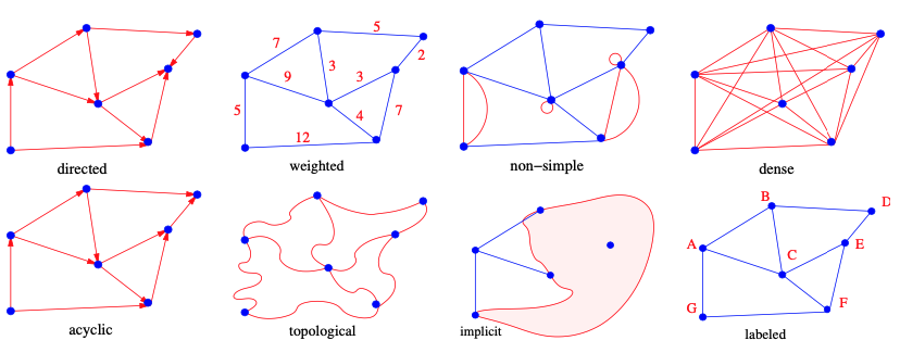
Type of graphs
1. Undirected graphs
-
A graph $G=(V,E)$ is undirected if $(u,v) \in E$ implies $(v,u) \in E$.
- $(u,v) = (v,u)$
- i.e. friendship, etc.
-
Edges in undirected graphs:
- Tree edges
- discover new vertices.
- encoded in parent relation.
- Back edges
- point back into the tree.
- their other endpoint is an ancestor of the vertex being expanded.
- Tree edges
2. Directed graphs
- Directions are defined for edges.
- i.e. following someone on Twitter, etc.
3. Unweighted graphs
- There is no cost distinction between various edges and vertices.
- A shortest path can be found using BFS in unweighted graphs.
4. Weighted graphs
- Each edge is assigned a numerical value or weight.
5. Tree
- Undirected acyclic graph
6. Rooted tree
- Every edge either points away from or towards the root node.
7. Cyclic graphs
- A cycle is a closed path of 3 or more vertices that has no repeating vertices except the start/end point.
8. Acyclic graphs
- Graphs without cycles
9. Directed acyclic graph (DAG)
- Both directed and acyclic graphs
- Naturally arise in scheduling problems
- $(u,v)$ indicates that activity $u$ must occur before $v$.
- Topological sort is the first step of a DAG.
10. Bipartite graph
- Vertices can be split into two independent groups, $U$ and $V$, such that every edge connects between $U$ and $V$.
- It can be coloured without conflicts while using only two colours.
- It can only have an even edge length cycle.
11. Complete graph
- There is a unique edge between every pair of nodes.
12. Simple graph
- It does not contain more than one edge between the pair of vertices.
13. Non-simple graph
- It contains more than one edge between the pair of vertices.
14. Sparse graph
- Only a small fraction of the possible vertex pairs have edges defined between them.
15. Dense graph
- A large fraction of the vertex pairs define edges.
16. Embedded graph
- The vertices and edges are assigned geometric positions.
- Its drawing may or may not have algorithmic significance.
17. Topological graph
- Grid of points is an example.
18. Implicit graph
- The vertices of this implicit search graph are the states of the search vector, while edges link pairs of states that can be directly generated from each other. A web-scale analysis is another example, where you should try to dynamically crawl and analyze the small relevant portion of interest instead of initially downloading the entire web.
19. Explicit graph
- It is often easier to work with an implicit graph and store the entire thing before analysis.
20. Labelled graph
- Each vertex is assigned a unique name or identifier.
21. Unlabeled graph
- Each vertex is the same.
Graph visualization
- iGraph
- Graphviz
- MuxViz
- NetworkX
Independent set
Isomorphism
- Isomorphism testing determines whether the topological structures of two graphs are identical either respecting or ignoring any labels.
Maximum clique
Nearest neighbour
Negativity
- Does the weighted graph have any negative cycles? If so, where?
Negativity algorithms
- Bellman-Ford
- Floyd-Warshall
Paths
from typing import Dict, List

def dfs(graph: Dict[int, int], start_node: int) -> List[int]:
    stack = [start_node]
    visited = []
    while stack:
        popped_node = stack.pop()
        if popped_node not in visited:
            for neighbour in graph[popped_node]:
                if neighbour not in visited:
                    stack.append(neighbour)
            visited.append(popped_node)
    return visited

def bfs(graph: Dict[int, int], start_node: int) -> List[int]:
 visited = [start_node]
 queue = [start_node]
 while queue:
  popped_node = queue.pop(0)
  for neighbour in graph[popped_node]:
   if neighbour not in visited:
    queue.append(neighbour)
    visited.append(neighbour)
 return visited

def is_path(graph: Dict[int, int], start_node: int, end_node: int) -> bool:
 if start_node == end_node:
  return True

 if end_node in bfs(graph, start_node): # bfs := path from start node
  return True

 return False

if __name__ == "__main__":

 letter_graph = { 'a' : ['d'],
     'b' : ['d', 'f'],
     'c' : [],
     'd' : ['a', 'b', 'e', 'f'],
     'e' : ['d'],
     'f' : ['b', 'd'],
     }

 # print(dfs(letter_graph, 'a'))
 # print(bfs(letter_graph, 'b'))
 # print(is_path(graph=letter_graph, start_node='a', end_node='e'))
 # print(is_path(graph=letter_graph, start_node='c', end_node='f'))
 # print(is_path(graph=letter_graph, start_node='f', end_node='f'))
Strongly connected components
- Self-contained cycles within a directed graph where every vertex in a given cycle can reach every other vertex in the same cycle.
- i.e. Road networks, otherwise there will be places you can drive to but not drive home from without violating one-way signs.
Kosaraju’s
- Two-pass algorithm
- DFS
- Order by finish time in decreasing order
from typing import List, Tuple

class Graph:
    def __init__(self, edge_list: List[Tuple[int, int]]):
        self.graph = {}
        for (src, dest) in edge_list:
            if src not in self.graph:
                self.graph[src] = []
            if dest not in self.graph:
                self.graph[dest] = []
            self.graph[src].append(dest)

    def reverse_graph(self):
        rev = {}
        for src in self.graph:
            for dest in self.graph[src]:
                if src not in rev:
                    rev[src] = []
                if dest not in rev:
                    rev[dest] = []
                rev[dest].append(src)
        return rev

    def dfs(self, node, visited, departure):
        visited.append(node)
        for neig in self.graph[node]:
            if neig not in visited:
                self.dfs(neig, visited, departure)
        departure.append(node)

    def get_component(self, node, visited, component, rev_g):
        component.append(node)
        visited.append(node)
        for neig in rev_g[node]:
            if neig not in visited:
                self.get_component(neig, visited, component, rev_g)

    def strongly_connected_component(self):
        departure = [] # order of departure is the departure time
        visited = []
        for node in self.graph:
            if node not in visited:
                self.dfs(node, visited, departure)

        rev_g = self.reverse_graph()

        res = []
        visited = []
        while departure:
            node = departure.pop()
            if node not in visited:
                component = []
                self.get_component(node, visited, component, rev_g)
                res.append(component)
        return res


if __name__ == '__main__':
    edge_list = [ (0,1), (1,2), (2,0), (1,3), (3,4), (4,5), (5,3), (5,6) ]
    g = Graph(edge_list)
    print(g.strongly_connected_component())
Tarjan’s
- It can be used to find cycles in a graph.
Topological Sort (Top Short)
-
The most important operation on DAG
-
Topology is the way the parts of something are arranged and related.
-
There can be more than one topological sorting for a graph.
-
There is an ordering on the nodes of the graph, for every directed edge $(u,v)$, vertex $u$ comes before $v$ in the ordering.
- i.e. School class prerequisites, etc.
-
Topological orderings are NOT unique.
-
Runtime: $O(V+E)$
Topological sort algorithm
- Find an unvisited node
- Begin with the selected node, and do a DFS exploring only unvisited nodes.
- On the recursive callback of the DFS, add the current node to the topological ordering in reverse order.
class Graph:
    def __init__(self, edges, order):
        self.order = order
        self.adj_list = {}
        for (src, dest) in edges:
            if src not in self.adj_list:
                self.adj_list[src] = []
            if dest not in self.adj_list:
                self.adj_list[dest] = []
            self.adj_list[src].append(dest)

    def dfs(self, node, visited):
        if node not in visited:
            visited.append(node)
            for neighbour in self.adj_list[node]:
                self.dfs(neighbour, visited)
            stack.append(node) # back

if __name__ == '__main__':
    edges = [ (0, 6), (1, 2), (1, 4), (1, 6), (3, 0), (3, 4), (5, 1), (7, 0), (7, 1) ]
    graph = Graph(edges, 8)
    visited = []
    stack = []
    for node in graph.adj_list:
        graph.dfs(node, visited)
    print(visited)
    print(stack)
Two colouring
from collections import defaultdict

def dfs(node, g):
 if node in visited:
  return visited[node] == g
 visited[node] = g
 return all(dfs(neighbour,1-g) for neighbour in graph[node])


if __name__ == "__main__":
 # dislikes = [ [1,2], [1,3], [2,3], [3,4] ]
 dislikes = [ [1,2], [1,3], [3,4] ]

 graph = defaultdict(list)

 for node in dislikes:
  graph[node[0]].append(node[1])
  graph[node[1]].append(node[0])

 visited = {}
 print(all(dfs(node,0) for node in graph if node not in visited))
Union
class DisjointSet:

 def __init__(self, size):
  self.root = [i for i in range(size)]

 def find(self, x):
  return self.root[x]

 def union(self, x, y):
  rootX = self.find(x)
  rootY = self.find(y)
  if rootX != rootY:
   for i in range(len(self.root)):
    if self.root[i] == rootY:
     self.root[i] = rootX

 def is_connected(self, x, y):
  return self.find(x) == self.find(y)

 def __repr__(self):
  return str(self.root)


if __name__ == "__main__":

 disjoint_set = DisjointSet(size=10)
 disjoint_set.union(1, 2)
 disjoint_set.union(2, 5)
 disjoint_set.union(5, 6)
 disjoint_set.union(6, 7)
 disjoint_set.union(3, 8)
 disjoint_set.union(8, 9)
 print(disjoint_set.is_connected(1, 5))  # true
 print(disjoint_set.is_connected(5, 7))  # true
 print(disjoint_set.is_connected(4, 9))  # false
 # 1-2-5-6-7 3-8-9-4
 disjoint_set.union(9, 4)
 print(disjoint_set.is_connected(4, 9))  # true
Union by rank
class DisjointSet:

 def __init__(self, size):
  self.root = [i for i in range(size)]
  self.rank = [1 for i in range(size)]

 def find(self, x):
  while x != self.root[x]:
   x = self.root[x]
  return x

 def union(self, x, y):
  rootX = self.find(x)
  rootY = self.find(y)
  if rootX != rootY:
   if self.rank[rootX] > self.rank[rootY]:
    self.root[rootY] = rootX
   elif self.rank[rootX] < self.rank[rootY]:
    self.root[rootX] = rootY
   else:
    self.root[rootY] = rootX
    self.rank[rootX] += 1

 def __repr__(self):
  return str(self.root)
if __name__ == "__main__":

 disjoint_set = DisjointSet(10)

 disjoint_set.union(1, 2)
 disjoint_set.union(2, 5)
 disjoint_set.union(5, 6)
 disjoint_set.union(6, 7)
 disjoint_set.union(3, 8)
 disjoint_set.union(8, 9)
 disjoint_set.union(9, 4)
 print(str(disjoint_set))
Unweighted graphs
Hamiltonian cycle
- Does there exist a simple tour that visits each vertex of an unweighted graph
Gwithout repetition?
Vertex cover
Walk, Path, and Circuit
Walk (Trail)
- Finite alternative sequence of vertices and edges.
- No edge can appear more than once in the sequence.
- i.e., $v_k$ $e_m$ $v_n$ …
- Walk
- open
- closed $\rightarrow$ terminal vertex: initial and final vertex
Path
- An open walk in which no vertex can appear more than once.
Circuit
- A closed walk at least one edge in which no vertex except the terminal vertices appears more than once.
Weighted graphs
Maximum flow (Network flow)
- With an infinite input source, how much flow can we push through the network?
- Traditional algorithms are based on the idea of augmenting paths.
Algorithms
- Ford-Fulkerson
- Edmonds-Karp
- Dinic’s
Ford Fulkerson
-
Greedy
-
Runtime:
- $O(VE^2)$ with BFS (Edmonds-Karp)
- $O(V^3)$ with adjacency matrix
-
Terminologies
- Augmenting Path is the path available in a flow network.
- Residual Graph represents the flow network that has additional possible flow.
- Residual Capacity is the capacity of the edge after subtracting the flow from the maximum capacity.
- Minimum cut
-
Steps
- Initialize the flow in all the edges to 0.
- While there is an augmenting path between the source and the sink, add this path to the flow.
- Update the residual graph.
-
Applications
- Water distribution pipeline
- Bipartite matching problem
- Circulation with demands
from collections import defaultdict

class Graph:

    def __init__(self, graph):
        self.graph = graph

    def bfs(self, s, t, parent):
        visited = [s]
        queue = [s]
        while queue:
            u = queue.pop(0)
            for ind,val in enumerate(self.graph[u]):
                if ind not in visited and val > 0:
                    queue.append(ind)
                    visited.append(ind)
                    parent[ind] = u
        return t in visited

    def ford_fulkerson(self, source, sink):
        parent = [-1] * len(self.graph)
        max_flow = 0
        while self.bfs(source, sink, parent):

            s = sink
            path_flow = float("inf")
            while s != source:
                path_flow = min(path_flow, self.graph[parent[s]][s])
                s = parent[s]
            max_flow += path_flow

            v = sink
            while v != source:
                u = parent[v]
                self.graph[u][v] -= path_flow
                self.graph[v][u] += path_flow
                v = parent[v]

        return max_flow

g = Graph( [[0, 8, 0, 0, 3, 0],
            [0, 0, 9, 0, 0, 0],
            [0, 0, 0, 0, 7, 2],
            [0, 0, 0, 0, 0, 5],
            [0, 0, 7, 4, 0, 0],
            [0, 0, 0, 0, 0, 0], ])

print("Max Flow: %d " % g.ford_fulkerson(source=0, sink=5))
Edmonds Karp
- Uses a BFS as a method of finding augmenting paths
- Runtime:
$O(E^2V)$
Dinic
- Uses a combination of BFS + DFS to find augmenting paths
- $O(V^2E)$
Capacity scaling
- Adds a heuristic on top of Ford-Fulkerson to pick larger paths first
- Runtime: $O(E^2log(U))$
Push relabel
- Uses a concept of maintaining a “preflow” instead of finding augmenting paths to achieve a max-flow solution
- Runtime: $O(V^2E)$ or $V^2\sqrt{E}$
Min-cut
Minimum spanning trees
- A spanning tree is a subgraph of the undirected connected graph with the minimum possible number of edges.
- The subgraph should contain each node of the original graph.
- The spanning tree in which the sum of edges is minimum as possible then that spanning tree is called the minimum spanning tree.
- A graph can have multiple spanning-tree but it can have only one unique minimum spanning tree.
- Connected and acyclic
- The cheapest smallest possible network
- The minimum spanning tree of a graph is unique if all
medge weights in the graph are distinct.
Minimum spanning trees algorithms
- Kruskal’s
- Prim’s
- Boruvka’s
Boruvka’s
Kruskal’s
- Runtime: $O(ElogV)$ with binary heaps
- Runtime: $O(E+VlogV)$ with Fibonacci heaps
- Select the least costly node until the end.
- Selection order doesn’t matter for the nodes with the same cost.
- Greedy algorithm
Kruskal’s algorithm steps
- Sort all the edges in non-decreasing order of their weight.
- Pick the smallest edge. Check if it forms a cycle with the spanning tree formed so far. If a cycle is not formed, include this edge. Else, discard it.
- Repeat step 2 until there are $order-1$ edges in the spanning tree.
- Repeatedly add the next lightest edge that doesn’t produce a cycle.
class Graph:

 def __init__(self, vertices):
  self.V = vertices
  self.graph = []

 def addEdge(self, u, v, w):
  self.graph.append([u, v, w])

 def find(self, parent, i):
  """ which set does i belong
  """
  if parent[i] == i:
   return i
  return self.find(parent, parent[i])

 def union(self, parent, rank, x, y):
  """ merge sets containing x and y
  """
  xroot = self.find(parent, x)
  yroot = self.find(parent, y)

  # Attach smaller rank tree under the root of high-rank tree
  if rank[xroot] < rank[yroot]:
   parent[xroot] = yroot
  elif rank[xroot] > rank[yroot]:
   parent[yroot] = xroot

  # If ranks are the same, then make one a root and increment its rank by one
  else:
   parent[yroot] = xroot
   rank[xroot] += 1

 def KruskalMST(self):

  result = []
  i, e = 0, 0
  self.graph = sorted(self.graph, key=lambda item: item[2])

  parent, rank = [], []
  for node in range(self.V):
   parent.append(node)
   rank.append(0)

  while e < self.V - 1:
   u, v, w = self.graph[i]
   i += 1
   x = self.find(parent, u)
   y = self.find(parent, v)
   if x != y:
    e += 1
    result.append([u, v, w])
    self.union(parent, rank, x, y)

  minimumCost = 0
  for u, v, weight in result:
   minimumCost += weight
   print("%d -- %d == %d" % (u, v, weight))
  print("Minimum Spanning Tree: " , minimumCost)

g = Graph(4)
g.addEdge(0, 1, 10)
g.addEdge(0, 2, 6)
g.addEdge(0, 3, 5)
g.addEdge(1, 3, 15)
g.addEdge(2, 3, 4)

g.KruskalMST()
Prim’s
-
Greedy algorithm
-
It starts with the single source node and later explores all the adjacent nodes of the source node with all the connecting edges. While we are exploring the graphs, we will choose the edges with the minimum weight and those which cannot cause the cycles in the graph.
-
Runtime:
- $O(V^2)$ adjacency matrix, searching
- $O(ElogV)$ binary heap and adjacency list
- $O(E+VlogV)$ Fibonacci heap and adjacency list
-
The algorithm is as given below:
- Initialize the algorithm by choosing the source vertex.
- Find the minimum weight edge connected to the source node and another node and add it to the tree.
- Keep repeating this process until we find the minimum spanning tree.
-
We create two sets of nodes:
- Visited nodes
- Unvisited nodes
class Graph:
     def __init__(self, order):
          self.V = order
          self.graph = [ [ 0 for column in range(order) ] for row in range(order) ]

     def printMST(self, parent):
          print("Edge \tWeight")
          for i in range(1, self.V):
               print (parent[i], "-", i, "\t", self.graph[i][parent[i]])

     def minKey(self, key, visited):
          min_ = float('inf')
          for v in range(self.V):
               if min_ > key[v] and v not in visited:
                    min_ = key[v]
                    min_index = v

          return min_index

     def primMST(self):
          key = [float('inf')] * self.V
          key[0] = 0

          parent = [None] * self.V
          parent[0] = -1

          visited = []
          for _ in range(self.V):
               u = self.minKey(key, visited)
               visited.append(u)

               for v in range(self.V):
                    if self.graph[u][v] > 0 and v not in visited and key[v] > self.graph[u][v]:
                         key[v] = self.graph[u][v]
                         parent[v] = u

          self.printMST(parent)

g = Graph(5)
g.graph = [ [0, 4, 0, 3, 5],
            [4, 0, 2, 0, 0],
            [0, 2, 0, 1, 0],
            [3, 0, 1, 0, 0],
            [5, 0, 0, 0, 0],
          ]

g.primMST()
Prim binary heap
from collections import defaultdict
import heapq

def create_spanning_tree(graph, starting_vertex):
    mst = defaultdict(set)
    visited = set([starting_vertex])
    edges = [ (cost, starting_vertex, to) for to, cost in graph[starting_vertex].items()]
    heapq.heapify(edges)

    while edges:
        cost, frm, to = heapq.heappop(edges)
        if to not in visited:
            visited.add(to)
            mst[frm].add(to)
            for to_next, cost in graph[to].items():
                if to_next not in visited:
                    heapq.heappush(edges, (cost, to, to_next))
    return mst

if __name__ == "__main__":
    example_graph = {
        'A': {'B': 2, 'C': 3},
        'B': {'A': 2, 'C': 1, 'D': 1, 'E': 4},
        'C': {'A': 3, 'B': 1, 'F': 5},
        'D': {'B': 1, 'E': 1},
        'E': {'B': 4, 'D': 1, 'F': 1},
        'F': {'C': 5, 'E': 1, 'G': 1},
        'G': {'F': 1},
    }

    print(create_spanning_tree(example_graph, 'A'))
Variations of minimum spanning trees
Low-degree spanning tree
Maximum spanning tree
- The maximum spanning tree can be found by negating the edge weights of the input graph G and using a minimum spanning tree algorithm on the result. The spanning tree of G that has the most negative weight will define the maximum-weight tree in G.
- i.e. Suppose an evil telephone company is contracted to connect a bunch of houses, such that they will be paid a price proportional to the amount of wire they install. Naturally, they will seek to build the most expensive possible spanning tree.
Minimum bottleneck spanning tree
Sometimes we seek a spanning tree that minimizes the maximum edge weight over all possible trees. Every minimum-spanning tree has this property. The proof follows directly from the correctness of Kruskal’s algorithm.
Such bottleneck-spanning trees have interesting applications when the edge weights are interpreted as costs, capacities, or strengths. A less efficient but conceptually simpler way to solve such problems might be to delete all “heavy” edges from the graph and ask whether the result is still connected. These kinds of tests can be done with BFS or DFS.
Minimum product spanning trees
Suppose we seek the spanning tree that minimizes the product of edge weights, assuming all edge weights are positive. Since $lg(a · b) = lg(a) + lg(b)$, the minimum spanning tree on a graph whose edge weights are replaced with their logarithms gives the minimum product spanning tree on the original graph.
Minimum Steiner tree
Suppose we want to wire a bunch of houses together, but have the freedom to add extra intermediate vertices to serve as a shared junction.
Shortest path
- Given a weight graph, find the shortest path of edges from $u$ to $v$.
Shortest path algorithms
- BFS
- Dijkstra’s
- Bellman-Ford
- Floyd-Warshall
- A*, etc.
Bellman-Ford
Dijkstra
- It provides all shortest paths in a network with their lengths.
- Runtime: $O(n^2)$
Dijkstra algorithm
- Mark all nodes as temporary
- Assign $d_v$ to $\inf$ for $v \neq s$ and $d_s$ to 0.
- Choose a temporary node $u$ with the smallest path length.
- Mark $u$ as permanent.
- $d_v = min {d_v, d_u + w_{uv}}$ for every temporary node $v$ adjacent to $u$.
- If no temporary nodes are left, STOP.
def dijkstra(nodes, edges, source_index=0):
 path_lengths = { node: float('inf') for node in nodes }
 path_lengths[source_index] = 0

 adj_nodes = { node: {} for node in nodes }
 for (u,v), w_uv in edges.items():
  adj_nodes[u][v] = w_uv
  adj_nodes[v][u] = w_uv

 temporary_nodes = [ node for node in nodes ]
 while len(temporary_nodes) > 0:
  upper_bounds = { node: path_lengths[node] for node in temporary_nodes }
  u = min(upper_bounds, key=upper_bounds.get)

  temporary_nodes.remove(u)

  for v, w_uv in adj_nodes[u].items():
   path_lengths[v] = min(path_lengths[v], path_lengths[u] + w_uv)

 return path_lengths

nodes = list(range(6))
edges = { (0,1): 1.0, (0,2): 1.5, (0,3):2.0, (1,3): 0.5, (1,4): 2.5, (2,3): 1.5, (3,5): 1.0 }
print(dijkstra(nodes, edges, source_index=0))
Floyd-Warshall
-
Find all-pair shortest path problem from a given weighted graph
-
It generates a matrix, which will represent the minimum distance from any node to all other nodes in the graph.
-
DP
-
Runtime: $O(n^3)$ := All shortest path := Dijkstra for each node
-
Runtime: $O(n^3)$ := Floyd-Warshall
def floyd(G, nV):
    dist = { (u,v): float('inf') if u != v else 0 for u in range(nV) for v in range(nV) }
    dist = { (u,v): G[u][v] for u in range(nV) for v in range(nV) }

    for k in range(nV):
        dist = { (u,v): min(dist[(u,v)], dist[(u,k)] + dist[(k,v)]) for u in range(nV) for v in range(nV) }

    for u in range(nV):
        for v in range(nV):
            print(dist[(u,v)], end="  ")
        print(" ")

if __name__ == "__main__":
    INF = float('inf')
    G = [ [0,  5,   INF, INF],
          [50, 0,   15,  5  ],
          [30, INF, 0,   15 ],
          [15, INF, 5,   0  ],
        ]

    floyd(G, 4)
Traveling salesman
- Given all cities and the distances between each pair of cities, what is the shortest possible route that visits each city exactly once and returns to the original city?
NP-hard- It tries to find the most efficient route given a set of restrictions like the seven bridges in Euler’s problem.
- It is figuring out the most efficient way to travel between pairs of cities of specified distances.
Traveling salesman algorithms
- Held-Karp
- Branch-and-bound
- Many approximation algorithms